If one searches for the J2 contribution to change in longitude of the ascending node (LAN, \( \Omega \)) and argument of periapsis (APe\( \omega \)), the usual answer is some variation of
\[ \frac{\partial \Omega}{\partial t} = -3 \pi J_2 \left(\frac{R_E}{p}\right)^2 \cos i \cdot \frac{1}{T} \]
\[ \frac{\partial \omega}{\partial t} = \frac{3}{2} \pi J_2 \left(\frac{R_E}{p}\right)^2 \left(5 \cos^2 i - 1\right) \cdot \frac{1}{T} \]
with Earth radius \( R_E \), equatorial inclination \( i \), orbital period \( T \) and semi-latus rectum \( p = a \sqrt{1 - e^2} \) with semi-major axis \( a \) and eccentricity \( e \). So the change in LAN after e.g. 500 seconds is then:
\[ \Delta \Omega = -3 \pi J_2 \left(\frac{R_E}{p}\right)^2 \cos i \cdot \frac{500}{T} \].
This is even the equation given in the Orbiter Doc\Technotes\gravity.pdf.
This works well for circular orbits, or for integer multiples of orbits, but breaks down for elliptical orbits (\( 0 < e < 1 \)), or hyperbolic orbits (\( 1 < e \)) for that matter. This is because the perturbation is proportional to the force of gravity, which itself is strongest at perigee and weakest at apogee.
I've looked online, and found these two publications: Kozai - Motion of a close Earth satellite and Sauer - Perturbations of a Hyperbolic Orbit. But I can't get either of them to work.

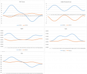
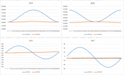
Here, in my MFD map, the green is the unperturbed orbit, yellow is with time fraction, purple is with TrA fraction (\(\frac{\nu -\nu_0}{2 \pi}\)), red is Kozai and light gray is Sauer.
We can see that over three orbits, none of the implementations accurately predict the final position.
So the question is: is it at all possible to find the total change in the elements over the next \( t \) seconds analytically? Or do I have to do some kind of iteration, and if so how?
The code of my implementation is
I know this is a highly technical question, so I will allow myself to tag @MontBlanc2012 directly, as I assume that is one of the few who can give an answer. But I'm of course welcoming any answer from anybody else too.
\[ \frac{\partial \Omega}{\partial t} = -3 \pi J_2 \left(\frac{R_E}{p}\right)^2 \cos i \cdot \frac{1}{T} \]
\[ \frac{\partial \omega}{\partial t} = \frac{3}{2} \pi J_2 \left(\frac{R_E}{p}\right)^2 \left(5 \cos^2 i - 1\right) \cdot \frac{1}{T} \]
with Earth radius \( R_E \), equatorial inclination \( i \), orbital period \( T \) and semi-latus rectum \( p = a \sqrt{1 - e^2} \) with semi-major axis \( a \) and eccentricity \( e \). So the change in LAN after e.g. 500 seconds is then:
\[ \Delta \Omega = -3 \pi J_2 \left(\frac{R_E}{p}\right)^2 \cos i \cdot \frac{500}{T} \].
This is even the equation given in the Orbiter Doc\Technotes\gravity.pdf.
This works well for circular orbits, or for integer multiples of orbits, but breaks down for elliptical orbits (\( 0 < e < 1 \)), or hyperbolic orbits (\( 1 < e \)) for that matter. This is because the perturbation is proportional to the force of gravity, which itself is strongest at perigee and weakest at apogee.
I've looked online, and found these two publications: Kozai - Motion of a close Earth satellite and Sauer - Perturbations of a Hyperbolic Orbit. But I can't get either of them to work.
Here, in my MFD map, the green is the unperturbed orbit, yellow is with time fraction, purple is with TrA fraction (\(\frac{\nu -\nu_0}{2 \pi}\)), red is Kozai and light gray is Sauer.
We can see that over three orbits, none of the implementations accurately predict the final position.
So the question is: is it at all possible to find the total change in the elements over the next \( t \) seconds analytically? Or do I have to do some kind of iteration, and if so how?
The code of my implementation is
C++:
double J2 = oapiGetPlanetJCoeff(ref, 0); // 0 gives J2.
// "Default" fraction of orbital period:
if (perturbation == 1)
{
    APe += 3.0 * PI2 / 4.0 * pow(refRad / el.a, 2.0) * (5.0 * cos(el.i) * cos(el.i) - 1.0) / pow(1.0 - el.e * el.e, 2.0) * J2 * t / prm.T;
    LAN += -3.0 * PI2 / 2.0 * pow(refRad / el.a, 2.0) * cos(el.i) / pow(1.0 - el.e * el.e, 2.0) * J2 * t / prm.T;
}

// My adaptation with fraction of TrA
if (perturbation == 2)
{
    double semiLatusRectum = el.a * (1.0 - el.e * el.e);
    double TrA0 = prm.TrA;
    APe += 3.0 * PI2 / 4.0 * refRad * refRad / semiLatusRectum / semiLatusRectum * (5.0 * cos(el.i) * cos(el.i) - 1.0) * J2 * (TrA - TrA0) / PI2;
    LAN += -3.0 * PI2 / 2.0 * refRad * refRad / semiLatusRectum / semiLatusRectum * cos(el.i) * J2 * (TrA - TrA0) / PI2;
}

// Kozai:
if (perturbation == 3)
{
    double sin2i = sin(el.i) * sin(el.i);
    double e2 = el.e * el.e;
    double semiLatusRectum = el.a / refRad * (1.0 - e2);
    double meanMotion = PI2 / prm.T;
    double semi2 = semiLatusRectum * semiLatusRectum;

    double dOmegaS = -J2 / semi2 * cos(el.i) * (TrA0 - MnA + el.e * sin(TrA0) - 0.5 * sin(2.0 * (APe + TrA0)) - el.e / 2.0 * sin(TrA0 + 2.0 * APe) - el.e / 6.0 * sin(3.0 * TrA0 + 2.0 * APe)); // unsure if TrA0 and MnA0 or for time t.
    double meanCos2TrA = (-el.e / (1.0 + sqrt(1.0 - e2))) * (-el.e / (1.0 + sqrt(1.0 - e2))) * (1.0 + 2.0 * sqrt(1.0 - e2)); // (11)
    double meanDOmegaS = -1.0 / 6.0 * J2 / semi2 * cos(el.i) * meanCos2TrA * cos(2.0 * APe); // (12)
    double OmegaDot = -J2 / semi2 * meanMotion * cos(el.i) * (1.0 + J2 / semi2 * (1.5 + e2 / 6.0 - 2.0 * sqrt(1.0 - e2) - sin2i * (5.0 / 3.0 - 5.0 / 24.0 * e2 - 3.0 * sqrt(1.0 - e2))));
    double dOmega1 = meanDOmegaS - J2 / semi2 * e2 * cos(el.i) / (2.0 * (4.0 - 5.0 * sin2i)) * ((7.0 - 15.0 * sin2i) / 6.0 + 5.0 * sin2i / (2.0 * (4.0 - 5.0 * sin2i)) * (14.0 - 15.0 * sin2i) / 6.0) * sin(2.0 * APe);
    LAN += OmegaDot * t + dOmegaS - meanDOmegaS + dOmega1;

    double domegaS = J2 / semi2 * ((2.0 - 2.5 * sin2i) * (TrA - MnA + el.e * sin(TrA)) \
        + (1.0 - 1.5 * sin2i) * (1.0 / el.e * (1.0 - 0.25 * el.e) * sin(TrA) + 0.5 * sin(2.0 * TrA) + el.e / 12.0 * sin(3.0 * TrA)) \
        - 1.0 / el.e * (0.25 * sin2i + (0.5 - 15.0 / 16.0 * sin2i) * e2) * sin(TrA + 2.0 * APe) + el.e / 16.0 * sin2i * sin(TrA - 2.0 * APe) \
        - 0.5 * (1.0 - 2.5 * sin2i) * sin(2.0 * (TrA + APe)) + 1.0 / el.e * (7.0 / 12.0 * sin2i - 1.0 / 6.0 * (1.0 - 19.0 / 8.0 * sin2i) * e2) * sin(3.0 * TrA + 2.0 * APe) \
        + 3.0 / 8.0 * sin2i * sin(4.0 * TrA + 2.0 * APe) + el.e / 16.0 * sin2i * sin(5.0 * TrA + 2.0 * APe));
    double meanDomegaS = J2 / semi2 * (sin2i * (0.125 + (1.0 - e2) / 6.0 / e2 * meanCos2TrA) + 1.0 / 6.0 * cos(el.i) * cos(el.i) * meanCos2TrA) * sin(2.0 * APe);
    double omegaDot = J2 / semi2 * meanMotion * (2.0 - 2.5 * sin2i) * (1.0 + J2 / semi2 * (2.0 + e2 / 2.0 - 2.0 * sqrt(1.0 - e2) - sin2i * (43.0 / 24.0 - e2 / 48.0 - 3.0 * sqrt(1.0 - e2)))) - 5.0 / 12.0 * J2 * J2 / semi2 / semi2 * e2 * meanMotion * pow(cos(el.i), 4); // (28)
    double domega1 = meanDomegaS - 3.0 / 8.0 * J2 / semi2 * sin2i * sin(2.0 * APe) - J2 / semi2 * (1.0 / (4.0 - 5.0 * sin2i) * ((14.0 - 15.0 * sin2i) / 24.0 * sin2i - e2 * (28.0 - 158.0 * sin2i + 135.0 * sin2i * sin2i) / 48.0) - e2 * sin2i * (13.0 - 15.0 * sin2i) / (4.0 - 5.0 * sin2i) / (4.0 - 5.0 * sin2i) * (14.0 - 15.0 * sin2i) / 24.0) * sin(2.0 * APe); // (30)
    APe += omegaDot * t + domegaS - meanDomegaS + domega1; // (31)
}

// Sauer:
if (perturbation == 4)
{
    double LANangleDiff = 6.0 * (TrA + el.e * sin(TrA)) - (3.0 * el.e * sin(2.0 * APe + TrA) + 3.0 * sin(2.0 * APe + 2.0 * TrA) + el.e * sin(2.0 * APe + 3.0 * TrA));
    LANangleDiff -= 6.0 * (TrA0 + el.e * sin(TrA0)) - (3.0 * el.e * sin(2.0 * APe + TrA0) + 3.0 * sin(2.0 * APe + 2.0 * TrA0) + el.e * sin(2.0 * APe + 3.0 * TrA0));
    double DeltaLAN = -J2 * cos(el.i) / 4.0 / pow(el.a / refRad * (1.0 - el.e * el.e), 2) * LANangleDiff; // we'll use this in the APe perturbation
    LAN += DeltaLAN;

    double APeAngleDiff = (1.0 - 1.5 * sin(el.i) * sin(el.i)) * (TrA + (4.0 + 3.0 * el.e * el.e) / (4.0 * el.e) * sin(TrA) + 0.5 * sin(2.0 * TrA) + el.e / 12.0 * sin(3.0 * TrA)) \
        - sin(el.i) * sin(el.i) / (48.0 * el.e) * (3.0 * el.e * el.e * sin(2.0 * APe - TrA) + (12.0 - 21.0 * el.e * el.e) * sin(2.0 * APe + TrA) - 36.0 * el.e * sin(2.0 * APe + 2.0 * TrA) \
            - (28.0 + 11.0 * el.e * el.e) * sin(2.0 * APe + 3.0 * TrA) - 18.0 * el.e * sin(2.0 * APe + 4.0 * TrA) - 3.0 * el.e * sin(2.0 * APe + 5.0 * TrA));
    APeAngleDiff -= (1.0 - 1.5 * sin(el.i) * sin(el.i)) * (TrA0 + (4.0 + 3.0 * el.e * el.e) / (4.0 * el.e) * sin(TrA0) + 0.5 * sin(2.0 * TrA0) + el.e / 12.0 * sin(3.0 * TrA0)) \
        - sin(el.i) * sin(el.i) / (48.0 * el.e) * (3.0 * el.e * el.e * sin(2.0 * APe - TrA0) + (12.0 - 21.0 * el.e * el.e) * sin(2.0 * APe + TrA0) - 36.0 * el.e * sin(2.0 * APe + 2.0 * TrA0) \
            - (28.0 + 11.0 * el.e * el.e) * sin(2.0 * APe + 3.0 * TrA0) - 18.0 * el.e * sin(2.0 * APe + 4.0 * TrA0) - 3.0 * el.e * sin(2.0 * APe + 5.0 * TrA0));
    APe += J2 * 3.0 / 2.0 / pow(el.a / refRad * (1.0 - el.e * el.e), 2) * APeAngleDiff - cos(el.i) * DeltaLAN;
}
I know this is a highly technical question, so I will allow myself to tag @MontBlanc2012 directly, as I assume that is one of the few who can give an answer. But I'm of course welcoming any answer from anybody else too.