van der Waals

[n72.75]

This sub-forum doesn't get enough posts, so I thought I'd share a matlab script and a graph or two.

I became interested in van der Waals equation recently after looking for ways to improve upon the ideal-gas based approach used in NASSP. This was much more of a tangent, than something I'd ever hope to implement, so don't worry, I'm not going to break it.

Here's the Wikipedia page for the van der Waals equation. https://en.wikipedia.org/wiki/Van_der_Waals_equation. Wikipedia explains it well, so I'll spare everyone my copying and pasting. The tl;dr is that ideal gasses to not consider molecular interaction; van der Waals models attractive and repulsive forces in fluids as a simple cubic equation.

Although not perfect, I was interested because of the ability to not only simulate processes in gas and liquid volumes, but also supercritical fluids and saturated vapor-liquid mixtures, and mixtures of different substances. Some things van der Waals predicts fairly poorly, it should be noted--steam for example--so my interest shifted fairly quickly towards the equation itself, and away from it qua a realistic representation of the physical world.

Computing state in the saturated vapor-liquid region is typically done using integration, iteratively. In searching for a non-iterative method, I found the work of Carl W. David of the University of Connecticut, and his equations for the vapor and liquid are interesting, and I'm not going to even attempt to LaTeX them into this post. Here's the paper https://opencommons.uconn.edu/cgi/viewcontent.cgi?article=1100&context=chem_educ

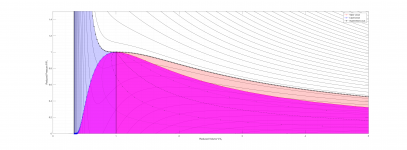
Below, is a graph showing a plot of reduced pressure and volume with different isotherms. The dotted and dashed lines in the saturated region show lines of constant vapor/liquid ratios (50%/50%, 75%/25%, etc.)

%Van der Waals
clear;
clc;

Tvdw = linspace(0,3.5,150);
V = linspace(0.25,5,202);

[TT,VV] = meshgrid(Tvdw,V);

P = 8/3.*(TT./(VV-1/3))-3./(VV.^2);
Pc = 8/3.*(1./(V-1/3))-3./(V.^2);


[Cplot,h1] = contourf(VV,P,TT,50);
##clabel(Cplot,h1);
colormap("white");
axis([0,5,0,1.5]);
grid minor;
xlabel("Reduced Volume V/V_c");
ylabel("Reduced Pressure P/P_c");

hold on

%the following equations are from %[1]

dd = linspace(0.001,25,200);
T = [length(dd)];
vg = [length(dd)];
vl = [length(dd)];
p = [length(dd)];

for ii = 1:length(dd)

d = dd(ii);
x = dd(ii);

vg(ii) = -1/6*(4*x*exp(2*x) - exp(4*x) + 1)*exp(x)/(x*exp(3*x) +...
x*exp(x) - exp(3*x) + exp(x)) + 1/3;

vl(ii) =-1/6*(4*x*exp(2*x) - exp(4*x) + 1)*exp(-x)/(x*exp(3*x) + x*exp(x) -
exp(3*x) + exp(x)) + 1/3;

T(ii) = -27/4*((4*d*exp(2*d) - exp(4*d) + 1)*((4*d*exp(2*d) - exp(4*d) + 1)*exp(-d)...
/(d*exp(3*d) + d*exp(d) - exp(3*d) + exp(d)) - 2)^2*exp(d)/(d*exp(3*d) + d*exp(d) -...
exp(3*d) + exp(d)) + (((4*d*exp(2*d) - exp(4*d) + 1)*exp(d)/(d*exp(3*d) + d*exp(d) -...
exp(3*d) + exp(d)) - 2)^2 + 4*(4*d*exp(2*d) - exp(4*d) + 1)*exp(d)/(d*exp(3*d) +...
d*exp(d) - exp(3*d) + exp(d)) - 4)*((4*d*exp(2*d) - exp(4*d) + 1)*exp(-d)/...
(d*exp(3*d) + d*exp(d) - exp(3*d) +...
exp(d)) - 2) + 2*((4*d*exp(2*d) - exp(4*d) + 1)*exp(d)/...
(d*exp(3*d) +...
d*exp(d) - exp(3*d) + exp(d)) - 2)^2 +...
4*(4*d*exp(2*d) - exp(4*d) + 1)*exp(d)/(d*exp(3*d) + d*exp(d) - exp(3*d) +...
exp(d)) - 8)/(((4*d*exp(2*d) - exp(4*d) +...
1)*exp(-d)/(d*exp(3*d) + d*exp(d) - exp(3*d) + exp(d)) - 2)^2*((4*d*exp(2*d) -...
exp(4*d) + 1)*exp(d)/(d*exp(3*d) + d*exp(d) - exp(3*d) + exp(d)) - 2)^2);

p(ii) = 8*T(ii)/(3*vg(ii)-1)-3/vg(ii)^2;
endfor

#you will have to adjust the "33" if you change the resolution of V
area(V(33:end),Pc(33:end),'facecolor','red','facealpha',0.2);
area(V(1:33),Pc(1:33),'facecolor','blue','facealpha',0.2);
area(vg,p,'facecolor','magenta','facealpha',0.75);
area(vl,p,'facecolor','magenta','facealpha',0.75);

h2 = plot(vg,p,'r-+');
h3 = plot(vl,p,'b-x');
h4 = plot(V,Pc,'k-*');

vg50 = (vg+vl)/2;
vg75 = (3*vg+vl)/4;
vg25 = (vg+3*vl)/4;
vg10 = (vg+9*vl)/10;
vg90 = (vg*9+vl)/10;

plot(vg25,p,'k:.');
plot(vg50,p,'k--');
plot(vg75,p,'k:.');
plot(vg10,p,'k:');
plot(vg90,p,'k:');

hold off
legend([h2,h3,h4],'Vapor Locus','Liquid Locus','Supercritical Locus');

%test properties
T_test = 0.5
V_test = 0.5

Tcrit = 154.6; %K
Pcrit = 5043; %kPa

vg_test = interp1(T,vg,T_test,"cubic")
vl_test = interp1(T,vl,T_test,"cubic")

p_test = 8*T_test/(3*vg_test-1)-3/vg_test^2

gas = (V_test-vl_test)/(vg_test-vl_test);
liquid = 1 - gas;

disp(['Gas = ',num2str(gas*100),'%']);
disp(['Liquid = ',num2str(liquid*100),'%']);
disp(['Temperture = ',num2str(T_test*Tcrit),'K']);
disp(['Pressure = ',num2str(p_test*Pcrit),'kPa']);


%References

%[1] https://opencommons.uconn.edu/cgi/viewcontent.cgi?article=1107&context=chem_educ

VanDerWaal.m

GitHub Gist: instantly share code, notes, and snippets.

gist.github.com

 

[Sbb1413]

I have learnt that no real gas perfectly follow the Boyle's law, Charles' law and Avogadro's law. The gases that perfectly follow such laws are called "ideal gases". Although such gases imaginary, they are useful to approximate the parameters of a given gas by using the simple \( PV = nRT \) equation, where \( R \) is the universal gas constant. The Van der Waals' equation is more accurate but more complicated way to measure the parameters of a given gas (you have to remember two Van der Waals' constants alongside the \( R \) constant, and I can call up the latter only as 0.082 L · atm · mol^-1 · K^-1).